Speed up your Gibbs sampler 40 times with Rcpp

When Gibbs sampling in R is slow, we can use Rcpp to speed it up by integrating C++ code into R. However, Rcpp code is harder to debug because we cannot run Rcpp code line-by-line like R. It’s paramount that we ensure the Rcpp code is doing what we wants it to.

The solution is to start with small Rcpp programs and make sure that they produce the same results as their pure R counterpart. Following this advice, I’m writing a series of increasingly complex Markov chain Monte Carlo (MCMC) code in Rcpp, eventually building towards my final goal of a custom Metropolis-Hastings algorithm for my work on modeling FDI flow.

The first installment will be a Gibbs sampler of a semi-conjugate normal model, arguably the most common introductory model to Bayesian statistics and MCMC. (Both Hoff’s First Course in Bayesian and Gelman’s Bayesian Data Analysis cover it.)

I’ll follow Hoff’s example in Chapter 6 as a ground truth to check whether my code is working correctly. For Rcpp basics, I read Hadley Wickham’s introduction to Rcpp. I’ll note additional pitfalls along the way of converting R to Rcpp.

Normal model with semi-conjugate priors

A normal model with semi-conjugate priors has the following specifications. For more details and intuition behind the model, see Chapter 5 & 6 in Hoff’s book.

Likelihood

\[Data = Y_1, \dots, Y_n \sim i.i.d. N(\theta, \sigma^2)\]

Priors

\[\begin{align} p(\theta) &\sim N(\mu_0, \tau^2_0) \\ p(\sigma^2) &\sim Inverse-Gamma(\nu_0 / 2, \nu_0 \sigma^2_0 / 2) \end{align}\]

Full conditionals

\[\begin{align} p(\theta | \tilde \sigma^2, Data) &= N(\mu_n, \tau^2_n) \\ p(\tilde \sigma^2 | \theta, Data) &= Inverse-Gamma(\frac{\nu_n}{2}, \frac{\nu_n \sigma_n^2(\theta)}{2}) \end{align}\]

with

\[\begin{align} \tau_n^2 = \frac{1}{\frac{1}{\tau_0^2} + \frac{n}{\sigma^2}} \qquad &\text{and} \qquad \mu_n = \frac{\frac{\mu_0}{\tau_0^2} + \frac{n\bar y}{\sigma^2}}{\frac{1}{\tau_0^2} + \frac{n}{\sigma^2}} \\ \nu_n = \nu_0 + n \qquad &\text{and} \qquad \sigma^2_n(\theta) = \frac{1}{\nu_n} \left[ \nu_0\sigma_0^2 + n \frac{\sum (y_i - \theta)^2}{n}\right] \end{align}\]

There is a quick intuitive interpretation of the full conditional of \(\theta\), \(p(\theta | \tilde\sigma^2, Data)\). Its posterior mean \(\mu_n\) is the weighted sum of the prior mean \(\mu_0\) and the sample mean \(\bar y\). This makes sense if we think of the posterior as combining the information from the prior and the sample.

But how should we weigh the information from the prior and the sample? Intuitively, if there’s more information in the prior, we should weigh it more. The amount of information in the prior is represented by the prior precision, \(\frac{1}{\tau_0^2}\). As the formula shows, the precision is the inverse of variance, because the smaller the variance there is in our prior belief about \(\theta\), the more information we have in the prior. In sum, because precision represents the amount of information available, we should weigh the prior mean \(\mu_0\) by the prior precision \(\frac{1}{\tau_0^2}\). That is indeed the weight of the prior mean in the weighted sum.

Similarly, we weigh the sample mean \(\bar y\) by the sample precision \(\frac{n}{\sigma^2}\). Note that we multiply the precision by \(n\) to capture the fact that the bigger the sample size, the more information there is in the sample.

Pure R Gibbs sampler

Below is a direct translation of the full conditionals below into a Gibbs sampler. Inside the big loop, for the iteration \(s\) we sample:

1. \[p(\theta^{(s)} | \tilde \sigma^{2(s - 1)}, Data)\]
2. \[p(\tilde \sigma^{2(s)} | \theta^{(s)}, Data)\]

and repeats.

f_gibbsR <- function(y, mu_0, tau2_0, sigma2_0, nu_0, S = 1000) {
  # Sample statistics
  n <- length(y) ; ybar <- mean(y)

  # Initialize storage
  res_theta <- rep(NA, S)
  res_sigma2 <- rep(NA, S)

  # Starting value as the sample variance and mean
  res_sigma2[1] <- var(y)
  res_theta[1] <- ybar
  
  # Gibbs sampler -- big loop
  for (s in 2:S) {
    # Full conditional for theta
    sigma2 <- res_sigma2[s - 1] # Get the current value of sigma2

    tau2_n <- 1 / (1 / tau2_0 + n / sigma2)
    mu_n <- (mu_0 / tau2_0 + n * ybar / sigma2) / (1 / tau2_0 + n / sigma2)

    # Generate and save theta. Note that rnorm takes SD, not variance
    res_theta[s] <- rnorm(1, mu_n, sqrt(tau2_n))

    # Full conditional for sigma
    theta <- res_theta[s] # Get the current value of theta

    nu_n <- nu_0 + n
    nu_sigma2_n <- nu_0 * sigma2_0 + sum((y - theta) ** 2)
    res_sigma2[s] <- 1 / rgamma(1, nu_n / 2, nu_sigma2_n / 2)
  }

  return(list(theta = res_theta, sigma2 = res_sigma2))
}

We confirm that our algorithm successfully reproduces the result in Hoff (p. 95) with exactly the same posterior distribution of theta.

# Data and priors are specified as in Hoff p. 95
y <- c(1.64,1.70,1.72,1.74,1.82,1.82,1.82,1.90,2.08)
set.seed(1)
gibbsR <- f_gibbsR(y = y, S = 1000,
                   mu_0 = 1.9, tau2_0 = 0.95 ** 2,
                   sigma2_0 = 0.01, nu_0 = 1)
quantile(gibbsR$theta, c(0.025, 0.5, 0.975)) # Exactly as in Hoff p. 95

##     2.5%      50%    97.5% 
## 1.707282 1.804348 1.901129

Rcpp Gibbs sampler

We now rewrite the Gibbs sampler in Rcpp. Putting the R and Rcpp codes side by side, we see only a few differences thanks to Rcpp’s syntactic sugar that replicates R-like syntax in C++. Most of these differences are covered in Hadley’s Intro to Rcpp. Beyond that, there are 2 additional pitfalls when transitioning from R to Rcpp.

1. Remember to use 1.0 instead of 1 while doing division so that we get double division like in R, not integer division. For example, in Rcpp, 1 / 2 = 0 while 1.0 / 2 = 0.5.

2. rgamma in R uses two parameters, location and rate. In contrast, rgamma in Rcpp uses location and scale, which is the inverse of rate.

#include <Rcpp.h>
using namespace Rcpp;

// [[Rcpp::export]]
List f_gibbsC(NumericVector y, int S,
                       double mu_0, double tau2_0,
                       double sigma2_0, double nu_0) {
  // Sample statistics
  double n = y.size();
  double ybar = mean(y);

  // Initialize storage
  NumericVector res_theta(S);
  NumericVector res_sigma2(S);

  // Starting value as the sample variance and mean
  res_sigma2[0] = var(y);
  res_theta[0] = ybar;

  // Gibbs sampler -- big loop
  // ATTENTION: We will still have S iterations, with s going from 0 to S - 1
  for (int s = 1; s < S; s++) {
    // Full conditional for theta
    double sigma2 = res_sigma2[s - 1];
    
    // ATTENTION: We use 1.0, instead of 1, so that we get double division instead of int
    double tau2_n = 1.0 / (1.0 / tau2_0 + n / sigma2);
    double mu_n = (mu_0 / tau2_0 + n * ybar / sigma2) / (1.0 / tau2_0 + n / sigma2);

    // Generate and save theta. Note that rnorm takes SD, not variance
    res_theta[s] = rnorm(1, mu_n, sqrt(tau2_n))[0];

    // Full conditional for sigma
    double theta = res_theta[s]; // Get the current value of theta

    double nu_n = nu_0 + n;
    double nu_sigma2_n = nu_0 * sigma2_0 + sum(pow((y - theta), 2));

    // Generate and save sigma2
    // ATTENTION: Unlike rgamma in R, rgamma in Rcpp use scale, not rate
    res_sigma2[s] = 1.0 / rgamma(1, nu_n / 2.0, 2.0 / nu_sigma2_n)[0];
  }

  List result; result["theta"] = res_theta ; result["sigma2"] = res_sigma2;
  return result;
}

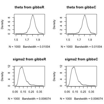
We now check and confirm that our Gibbs sampler in Rcpp produces exactly the same result as its pure R counterpart.

set.seed(1)
Rcpp::sourceCpp("gibbsC.cpp")
gibbsC <- f_gibbsC(y = y, S = 1000,
  mu_0 = 1.9, tau2_0 = 0.95 ** 2, sigma2_0 = 0.01, nu_0 = 1)

# Check if Rcpp result is the same as R
par(mfrow = c(2, 2))
plot(density(gibbsR$theta), main = "theta from gibbsR")
plot(density(gibbsC$theta), main = "theta from gibbsC")
plot(density(sqrt(gibbsR$sigma2)), main = "sigma2 from gibbsR")
plot(density(sqrt(gibbsC$sigma2)), main = "sigma2 from gibbsC")

Comparing the density plots on the left with those on the right, we see that the posterior distributions of \(\theta\) and \(\sigma^2\) are exactly the same for the R and Rcpp implementations.

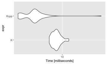
The Rcpp code is also a lot faster than R as expected. The median running time of f_gibbsC is about 38 times faster than f_gibbsR.

library(microbenchmark)
benchmark_result <- microbenchmark(
  f_gibbsR(y = y, S = 1000, mu_0 = 1.9, tau2_0 = 0.95 ** 2,
           sigma2_0 = 0.01, nu_0 = 1),
  f_gibbsC(y = y, S = 1000, mu_0 = 1.9, tau2_0 = 0.95 ** 2,
           sigma2_0 = 0.01, nu_0 = 1))

library(ggplot2)
autoplot(benchmark_result) + scale_x_discrete(labels = c("R", "Rcpp"))

## Scale for 'x' is already present. Adding another scale for 'x',
## which will replace the existing scale.

And that’s the one of the simplest Gibbs sampler in Rcpp. In the next installment we will implement the Metropolis-Hastings sampler in Rcpp. You can click on the categories Bayesian-sampler-in-Rcpp to find more entries in this series.