Gotta plot ‘em all!

While waiting for Pokemon Go to hit my region, I decided to try out the excellent Poke API. I then analyzed the Pokemon stats with Principal Component Analysis (PCA) to see how they relate to each other.

Download ‘em all

To get the data, I accessed the API with R’s httr package, downloading all the stats and sprites for the original 151 Pokemons. You can also skip this part by downloading the data directly from their github.

rm(list = ls())
packs <- c("httr", "ggplot2", "dplyr")
lapply(packs, library, character.only = TRUE)

# Get Gen 1 information
rgen1 <- GET("http://pokeapi.co/api/v2/generation/1")
cgen1 <- content(rgen1, "parsed")

# Extract all species of Gen 1 into a data frame
df_poke_gen1 <- do.call(rbind.data.frame, c(cgen1$pokemon_species, stringsAsFactors = FALSE))

# We will crawl through the urls of all species, seen here in the url column
head(df_poke_gen1)

# A function to crawl through the url and extract the Pokemon and its stats
f_getpokemon <- function(url) {
  c_species <- content(GET(url), "parsed")

  # For gen 1, there's only one variety of Pokemon per species, so we can simply extract
  # the first element in the varieties list
  url_pokemon <- c_species$varieties[[1]]$pokemon$url
  c_pokemon <- content(GET(url_pokemon), "parsed")

  stats <- sapply(c_pokemon$stats, function(stats) stats[["base_stat"]])
  names(stats) <- sapply(c_pokemon$stats, function(stats) stats[["stat"]][["name"]])

  for (i in seq_along(c_pokemon$types)) {
    if (c_pokemon$types[[i]][["slot"]] == 1) {
      type <- c_pokemon$types[[i]][["type"]][["name"]]
    }
  }

  return(c(name = c_pokemon$name, url = url_pokemon,
           id = c_pokemon$id, order = c_pokemon$order,
           type = type,
           weight = c_pokemon$weight,
           sprite = c_pokemon$sprites$front_default,
           as.list(stats)))
}

# Get all pokemons using the function above
l_pokemon <- lapply(df_poke_gen1$url, f_getpokemon)
df_pokemon <- do.call(rbind.data.frame, c(l_pokemon, stringsAsFactors = FALSE))
df_pokemon <- df_pokemon %>% arrange(id)
write.csv(df_pokemon, file = "pokemon_gen1.csv", row.names = FALSE)

# Get all the pokemon sprites
dir.create("pokemon_png")
mapply(download.file,
       url = df_pokemon$sprite,
       destfile = paste0("pokemon_png/", df_pokemon$name, ".png"),
       MoreArgs = list(mode = "wb"))

Use Principal Component Analysis (PCA) to decompose Pokemon’s stats

Each Pokemon has 6 stats: HP, Attack, Defense, Speed, Special Attack, and Special Defense. To get a glimpse into how the game designer assigns values to these stats, we use PCA to discover the latent factors that summarize them. These latent factors are called principal components.¹

# Load the packages
packs <- c("ggplot2", "dplyr", "png", "grid")
lapply(packs, library, character.only = TRUE)

# Read in the data
df_pokemon <- read.csv("pokemon_gen1.csv")

# Run PCA on the 6 stats
pca <- prcomp(df_pokemon[ , c("speed", "special.defense", "special.attack",
                              "defense", "attack", "hp")])

To see how much variance in Pokemon’s stats is explained by the principal components, we use the screeplot, which plots the variances explained on the y-axis and the number of the principal component on the x-axis. In this case, we see that the first two principal components capture about half of the variance.

screeplot(pca, type = "lines", main = "Scree plot")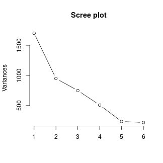

What do these two principal components represent? To understand their meaning, we project the 6 original stats onto the lower 2-dimensional space spanned by the two principal components. The 6 original stats are shown as the red vectors in the biplot below.

We see that all stats point to the right side of the the Principal Component 1 (PC1). So we could interpret PC1 as “Overall Strength”–the higher the value of PC1, the higher the value of all 6 stats.

On the other hand, along PC2, we see that HP, Attack, and Defense point to a different direction from that of Speed, Special Attack, and Special Defense. So we could interpret PC2 as some sort of “Brawn over Brain”–the higher the value of PC2, the higher the regular stats and the lower the special stats. (NB: Regular stats, e.g. Attack and Defense affect physical moves, while special stats, e.g. Speciall Attack and Special Defense affect elemental moves.)

As you can see, PC1 is pretty intuitive – one can guess from the outset that Pokemons should vary a lot based on their overall strength. To me what’s interesting is really PC2, which shows that the second most important way that Pokemons vary is along the Regular Stat-vs-Special Stat dimensions (which I call Brawn over Brain). That wasn’t something I expected before the analysis.

biplot(pca, cex = c(0.6, 0.85), arrow.len = 0.05,
       xlab = "PC1 - Overal Strength",
       ylab = "PC2 - Brawn over Brain")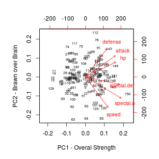

So here are the 151 Pokemons plotted on the space spanned by these two PCs. Mewtwo and Margikarp are, unsurprisingly, on the two extremes of the “Overall Strength” PC.

# Get the PCA data
pd <- cbind.data.frame(df_pokemon, pca$x)

# A function to plot Pokemon's png file as ggplot2's annotation_custom
f_annotate <- function(x, y, name, size) {
  f_getImage <- function(name) {
    rasterGrob(readPNG(paste0("pokemon_png/", name, ".png")))
  }
  annotation_custom(f_getImage(name),
                    xmin = x - size, xmax = x + size, 
                    ymin = y - size, ymax = y + size)
}

# Wrap everything in a plot function
f_plot <- function(pd) {
  ggplot(data = pd, aes(x = PC1, y = PC2)) +
    geom_text(data = pd, aes(label = name), 
              hjust = 0.5, vjust = -1, size = 3.5, alpha = 0.5) +
    mapply(f_annotate, x = pd$PC1, y = pd$PC2, name = pd$name, size = 10)  +
    theme_bw() +
    labs(x = "Overall Strength", y = "Brawn over Brain") +
    coord_cartesian(xlim = c(-100, 120), ylim = c(-90, 90))
}

# Plot all 151 Pokemons
f_plot(pd)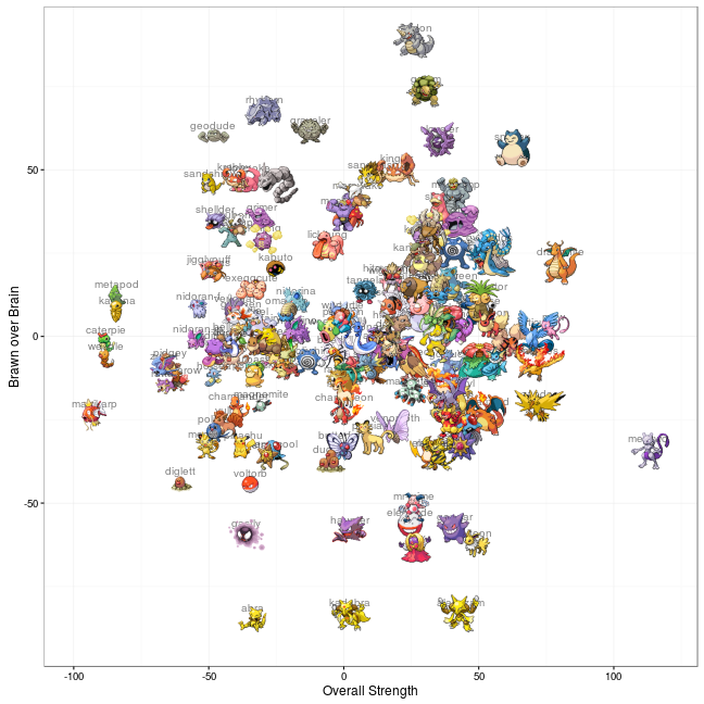

One way to think about PC2 is via the classic dilemma of choosing which Psychic pokemon for your team: Hypno or Alakazam. Looking at where these Pokemons position on the graph, we can see that both have similar overall strength (with Alakazam having slightly more). But along PC2, Alakazam places at the bottom of PC2, i.e. leaning heavily towards special stats at the exense of regular stats. On the other hand, Hypno has very balanced stats. That’s why lots of people choose Hypno as a robust Psychic type rather than the glass cannon that is Alakazam.

f_plot(pd %>% filter(name %in% c("abra", "kadabra", "alakazam",
                                 "drowzee", "hypno")))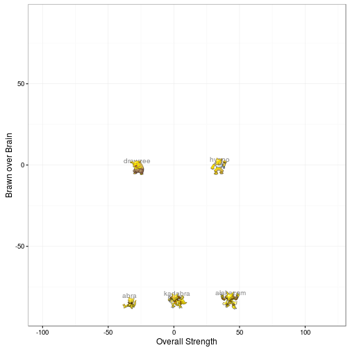

The three starter Pokemons are very balanced, with Charmander having a slight edge as it evolves to Charizard. If you squint really hard, it also seems like that strongest Pokemon at the first stage (Squirtle) turns out to be weakest at the final stage (Blatoise), and vice versa for Charmander and Charizard. That’s game balance design at work!

# Plot starter Pokemons
f_plot(pd %>% filter(id %in% 1:9))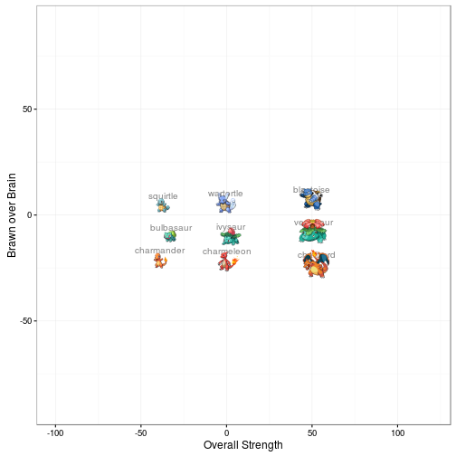

The final plot shows how Arcanine, my favorite Pokemon, rivals the Legendary birds in terms of stats. Indeed, Arcanine was planned to be a Legendary, but got changed before the game came out. Reddit has an entire thread devoted to this “Pokemon conspiracy”.

f_plot(pd %>% filter(name %in% c("arcanine", "moltres", "zapdos", "articuno")))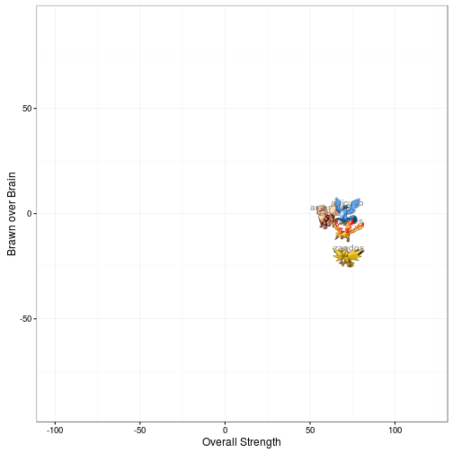

1. It’s recommended to normalize the data before running the PCA so that the variance of variables are not affected by the units that they are measured in. In this case it’s not necessary because Pokemon stats are all on the same scale. ↩